
摘要: Or Why You Should Use a Probabilistic Approach

▲來源:pixabay.com)
Most of the articles about AI predicting the stock markets focus on a more or less complicated model which tries to predict the move of the next timestep. And almost all of them are just focussing on architecture and layers like LSTM or CNN. But then they are just using the Mean Squared Error (MSE) as a loss function — and this is a problem and this article shows you why.
Somewhat State of The Art
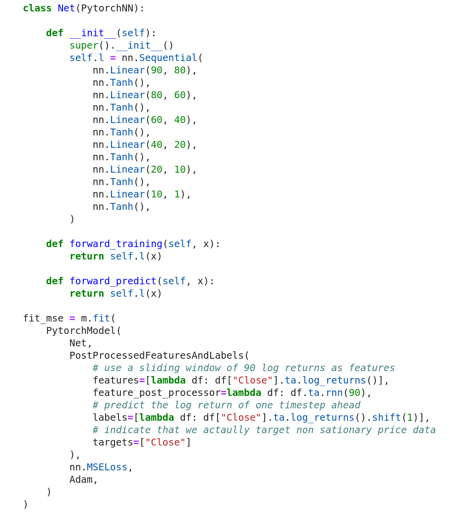
Assume we have the following Deep Neural Network (DNN) implemented in PyTorch. It is constructed arbitrarily but deep enough to simulate some level of a complex fancy architecture and has the following further properties:
- The input layer has 90 neurons because we are going to feed a moving window of 90 log returns as inputs
- The output layer has one single neuron which is supposed to predict the next day’s move
-
The model is fitted to a time series by using
* A moving window of 90 timesteps of log-returns (features + feature post-processor)
* The next timesteps log-return (labels) for the prediction
* Price reconstruction (target), which will later allow converting the stationary returns time series back to a non-stationary price time series for plotting
* The Mean Squared Error loss function
* And some optimizer (Adam)
Note that we use log returns because these should follow more closely a Normal Distribution which is an important detail for this article, as you will find out in a minute.
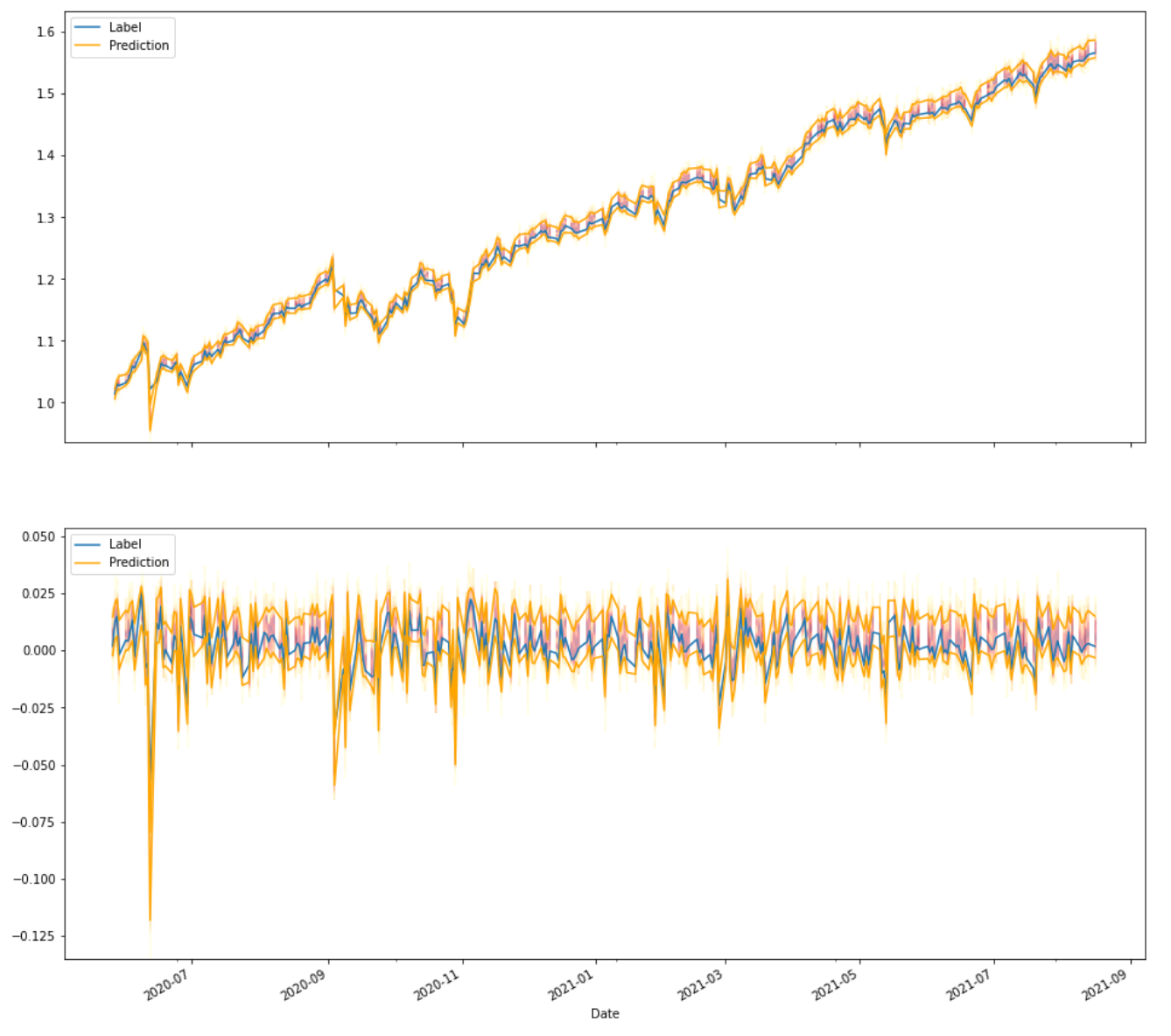
After the model got fitted to the SPY daily prices, it produced the following output for the test set. The orange line is the prediction while the blue line is the actual true event. And the orange shadow indicates the 80% confidence interval.
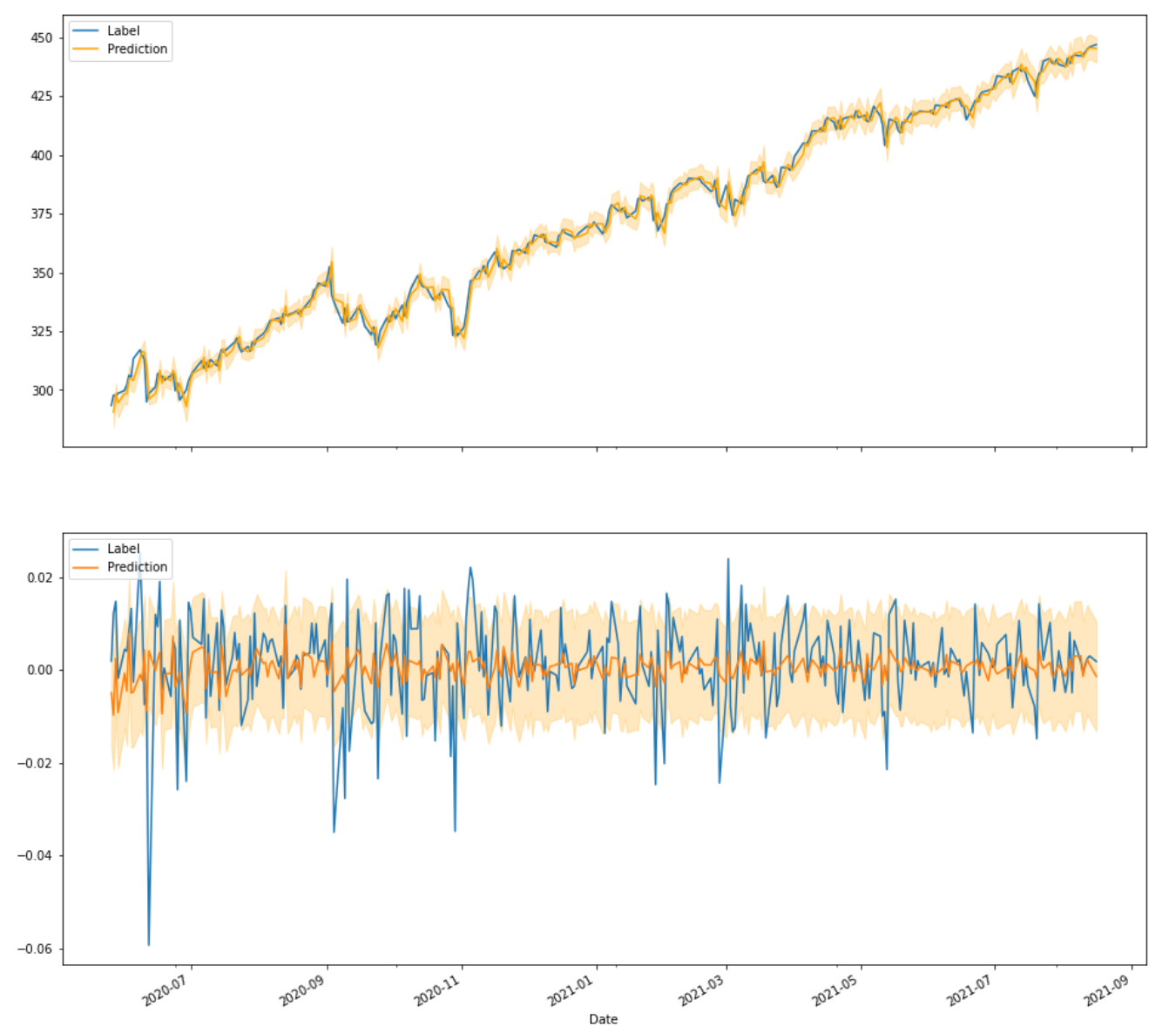
On the top, we see the reconstructed price time series and on the bottom, we see the return time series. By looking at the returns, what should be noted immediately is that the predictions themselves have much lower variance. By no means are they able to predict swings as big as we would expect from the true data. Then there is the confidence band which is constant and pretty wide (always ranging from negative to positive values). And there would be nothing different if you would add recurrent or convolutional layers. It does not matter how fancy the architecture of the network is, as long as a loss function with constant error is used, it will look very similar.
The Problem
As mentioned in the last sentence above: as long as a loss function with constant error is used, we will always get a similar result. Yes, the problem is actually the assumption of a constant error (aka variance).
Just by looking at the following picture of daily SPY returns, it should make sense that stock returns are not incorporating a constant variance [2].
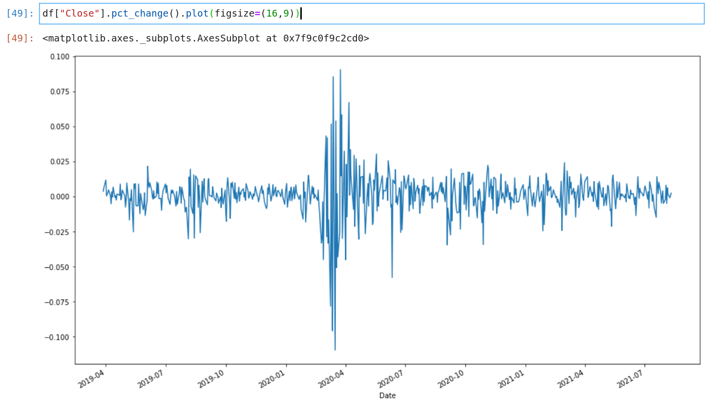
As a consequence, any standard MSE model will always overcompensate low volatility regimes and underestimate high volatility regimes, as volatility directly translates into variance (or standard deviation for that matter). It does not matter how accurate your model is, it will probably never predict a good signal. The reason is that the predictions will be always very close to zero and will have a huge variance.
To make this more visual, assume you have two models both of which predicting a +0.5% move for the next day. The first model has a standard deviation of 0.7% and the second one has a standard deviation of 0.5%. Model 1 would still lose 0.52% on average (hence more than the predicted gain) while model 2 on the other hand would only lose 0.45% on average.
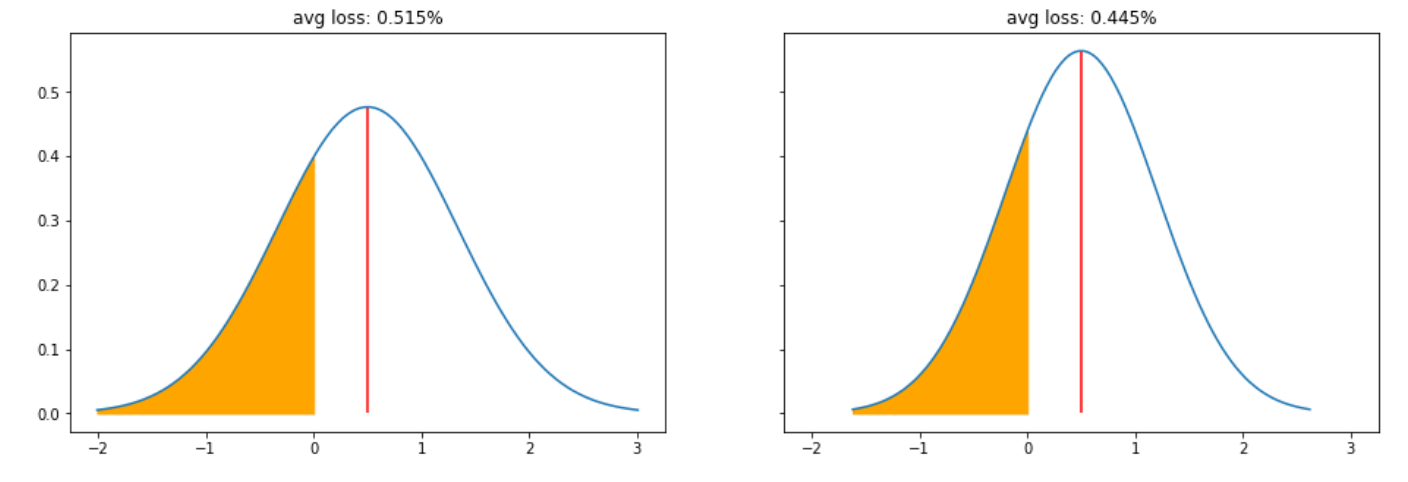
▲Average Loss (CVaR) of 0.7 vs 0.5 stddev
And yet it is well known that stock returns have fat tails, so the average losses will definitely be even higher. And this is the reason why basically any constant error model becomes kind of meaningless for stock return predictions, as the overall variance will be too high.
The MSE and the Normal Distribution
In order to fix this problem, we need to understand more of the details of the MSE loss. Take a look at the following two formulas. The first one is describing the variance of the Normal Distribution and the second one is the MSE.
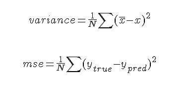
These two formulas look quite similar, right? And there is a reason for this. The simplest model using MSE loss is linear regression. What in fact happens by fitting a linear regression model, is that you are fitting a set of Normal Distributions, all with the same variance as demonstrated in the following picture.
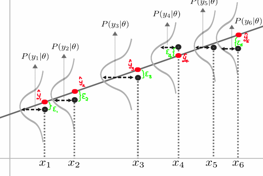
▲[1]
This is also easy to demonstrate in a small experiment:
- Sample a set of normally distributed random values (with a mean of zero and a given standard deviation)
- Add a trend to them
- And finally, fit a linear regression model and expect to get the same standard deviation back as the one used for the sampling in step 1
And this is exactly what happens (well, almost exactly but .456222… is pretty close to .456)
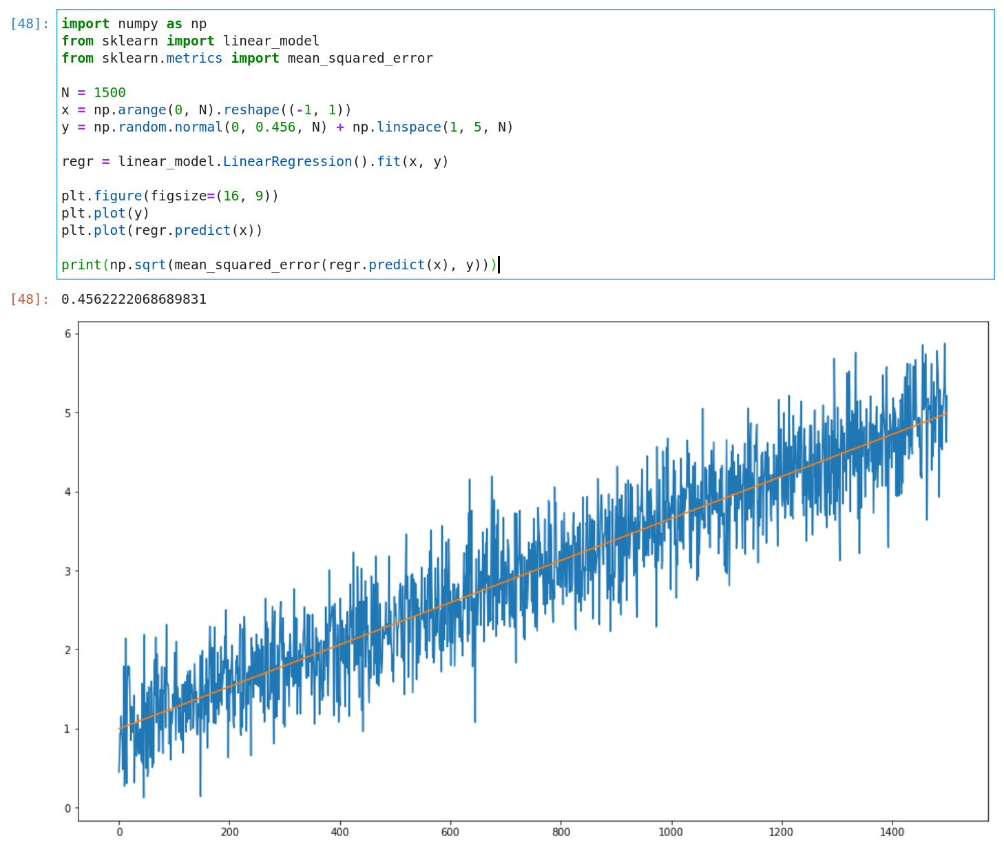
This means, whenever we predict a value ŷ we actually predict the mean of a Normal Distribution with a variance equal to the MSE loss of the fit. Or more generally: no matter how complex your model is (deep, recurrent or convolutional) as long as the optimized loss function is the MSE, your model will predict a mean of a Normal Distribution with the variance of the MSE.
Thinking Bayesian
While in a frequentist world it is good enough to say the expected value is ŷ, as a Bayesian this would not be a satisfying statement. Because by definition the true value will never be the predicted mean. To be precise, the probability of any exact value of any continuous distribution is always zero. This is why a Bayesian would say the predicted value will be any value following N(μ, σ) — a Normal Distribution with mean mu and standard deviation sigma.
The consequence of thinking bayesian is that you stop asking for a specific value like “what is the stock price of tomorrow”. Instead, you ask “what is the probability distribution of tomorrow's stock price”. And so far you have changed nothing, not a single bit of your model. However, only now (as a Bayesian) you are able to ask the right question: If stock returns do not follow a constant variance, how can I fit a model allowing a varying variance?
Go Probabilistic
Now we understand that we can only build a better model if we can handle varying variance (as opposed to constant variance). This should give the model the flexibility it needs to make better predictions under lower overall error (variance). The key to fit such a model is a different loss function, the Negative Log-Likelihood (NLL) loss. The NLL loss — very loosely speaking — allows the fitting of any kind of distribution, while we still want to stick to the Normal Distribution in this article.
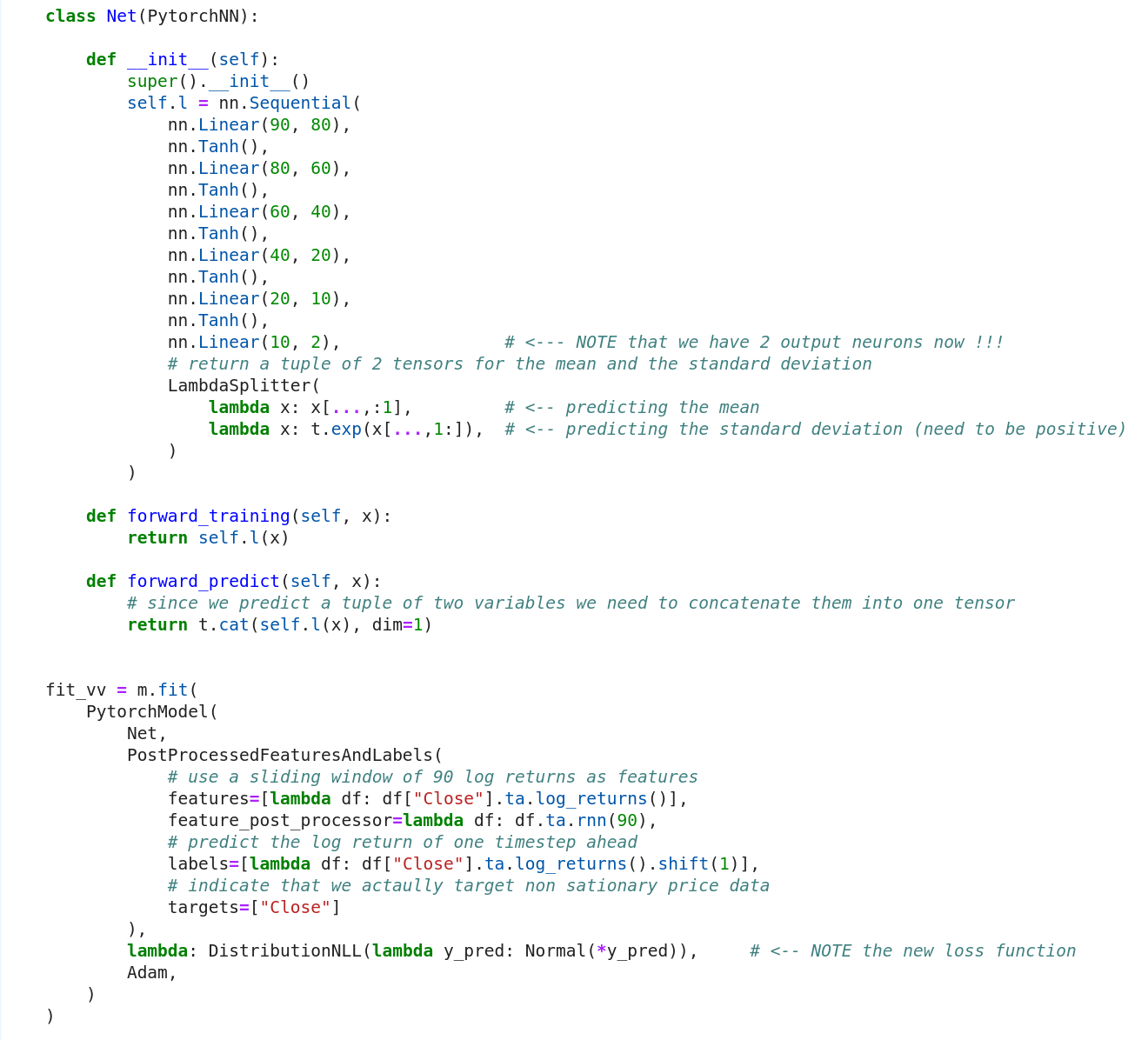
And here is what we need to turn our constant error model from the beginning into a probabilistic model:
- The last layer needs to output two neurons instead of one (μ and σ)
- The standard deviation (σ) can only be positive, so the last activation needs to be split into two functions where the exp function ensures the positivity
- Swap the MSE loss function with the NLL loss function to fit a Normal distribution (also provided by PyTorch)
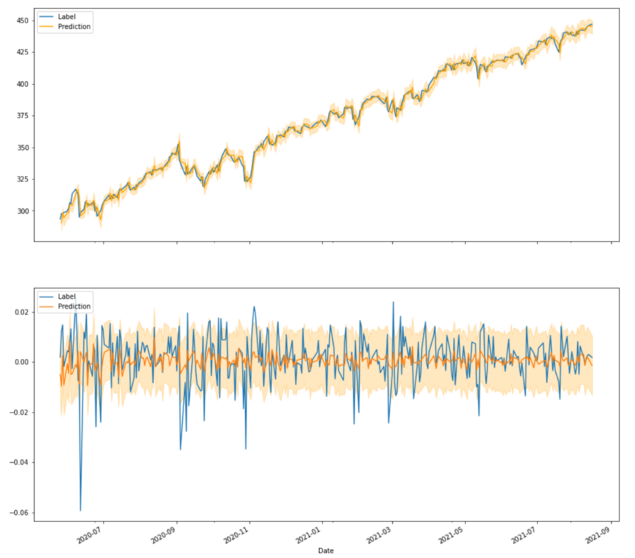
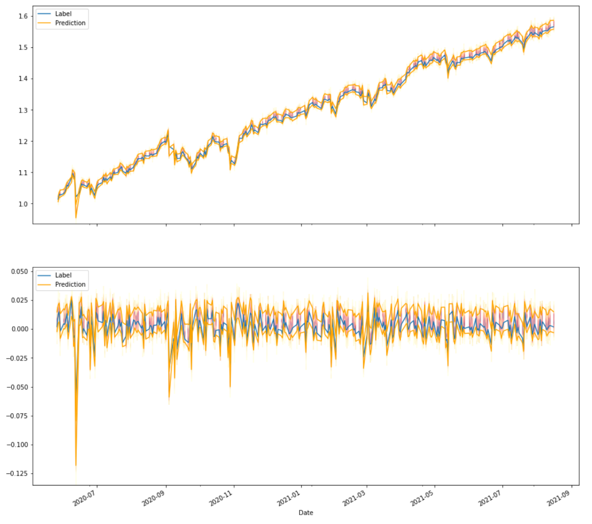
And this is what we get for the same time span of the test set as we got earlier. Even though the plot might look very noisy, it actually is much more accurate. The heat-map background shows the whole predicted distribution. And the 80% confidence band (now plotted as orange lines) is not behaving like a background anymore. The important thing to pay attention to is the fact, that the confidence band is more narrow overall and the true events (blue) are rarely outside of the confidence band (≤ 20% of the time ;-)).
Here we are, a model with varying variance predicting a Normal Distribution for the next time step where each of which has a different standard deviation. You can already see that there are more clear signals like the one in Sep 2020 where the whole confidence interval is negative. The model also adapts quickly to different volatility regimes like in Jun 2020 vs the last couple of months.
Conclusion
Time to draw some conclusions by comparing the two approaches side by side:
- The total variance of the probabilistic model is much smaller 0.006861 vs. 0.009227 (which is about a 3rd)
- The probabilistic model is also able to adapt to volatility regime changes while the constant error model is not (like in Jun 2020)
- The probabilistic model allows to fine-tune signals in terms of probabilities — like only go long when at least x% of the probability distribution is above 0
To be clear this is only a toy model for demonstration purposes, I would not trade either model at this point. But from now on you can not only fiddle with architecture and hyperparameters but also with various kinds of distributions. And Probabilistic models can add a whole new field to your trading ideas like market-neutral volatility strategies for example.
轉貼自Source: medium.com
若喜歡本文,請關注我們的臉書 Please Like our Facebook Page: Big Data In Finance

留下你的回應
以訪客張貼回應