
摘要: How to Build a Machine Learning Model Pipeline in Python
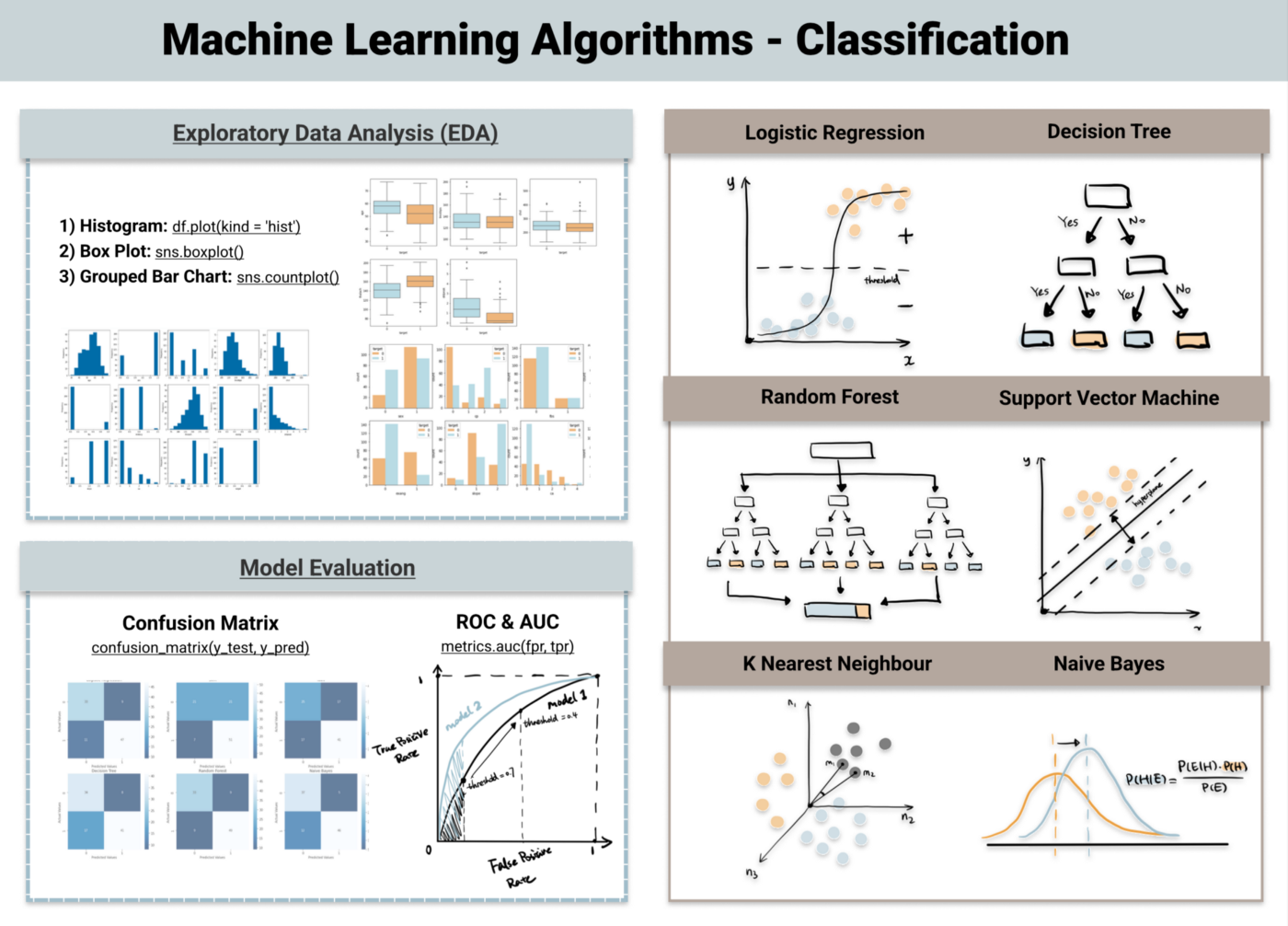
▲Machine Learning Algorithms for Classification (original image from my website)
Supervised vs. Unsupervised vs. Reinforcement Learning
The easiest way to distinguish a supervised learning and unsupervised learning is to see whether the data is labelled or not.
Supervised learning learns a function to make prediction of a defined label based on the input data. It can be either classifying data into a category (classification problem) or forecasting an outcome (regression algorithms).
Unsupervised learning reveals the underlying pattern in the dataset that are not explicitly presented, which can discover the similarity of data points (clustering algorithms) or uncover hidden relationships of variables (association rule algorithms) …
Reinforcement learning is another type of machine learning, where the agents learn to take actions based on its interaction with the environment, with the aim to maximize rewards. It is most similar to the learning process of human, following a trial-and-error approach.
Classification vs Regression
Supervised learning can be furthered categorized into classification and regression algorithms. Classification model identifies which category an object belongs to whereas regression model predicts a continuous output.
Sometimes there is an ambiguous line between classification algorithms and regression algorithms. Many algorithms can be used for both classification and regression, and classification is just regression model with a threshold applied. When the number is higher than the threshold it is classified as true while lower classified as false.
In this article, we will discuss top 6 machine learning algorithms for classification problems, including: logistic regression, decision tree, random forest, support vector machine, k nearest neighbour and naive bayes. I summarized the theory behind each as well as how to implement each using python. Check out the code for model pipeline on my website.
1. Logistic Regression
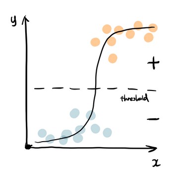
▲logistic regression (image by author)
Logistics regression uses sigmoid function above to return the probability of a label. It is widely used when the classification problem is binary — true or false, win or lose, positive or negative ...
The sigmoid function generates a probability output. By comparing the probability with a pre-defined threshold, the object is assigned to a label accordingly. Check out my posts on logistic regression for a detailed walkthrough.
Below is the code snippet for a default logistic regression and the common hyperparameters to experiment on — see which combinations bring the best result.
logistic regression common hyperparameters: penalty, max_iter, C, solver
2. Decision Tree
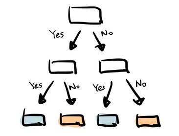
▲decision tree (image by author)
Decision tree builds tree branches in a hierarchy approach and each branch can be considered as an if-else statement. The branches develop by partitioning the dataset into subsets based on most important features. Final classification happens at the leaves of the decision tree.
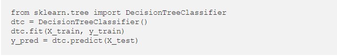
decision tree common hyperparameters: criterion, max_depth, min_samples_split, min_samples_leaf; max_features
3. Random Forest
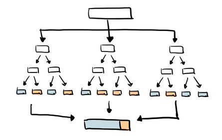
▲random forest (image by author)
As the name suggest, random forest is a collection of decision trees. It is a common type of ensemble methods which aggregate results from multiple predictors. Random forest additionally utilizes bagging technique that allows each tree trained on a random sampling of original dataset and takes the majority vote from trees. Compared to decision tree, it has better generalization but less interpretable, because of more layers added to the model.
random forest common hyperparameters: n_estimators, max_features, max_depth, min_samples_split, min_samples_leaf, boostrap
4. Support Vector Machine (SVM)
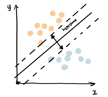
▲support vector machine (image by author)
Support vector machine finds the best way to classify the data based on the position in relation to a border between positive class and negative class. This border is known as the hyperplane which maximize the distance between data points from different classes. Similar to decision tree and random forest, support vector machine can be used in both classification and regression, SVC (support vector classifier) is for classification problem.
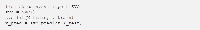
support vector machine common hyperparameters: c, kernel, gamma
5. K-Nearest Neighbour (KNN)
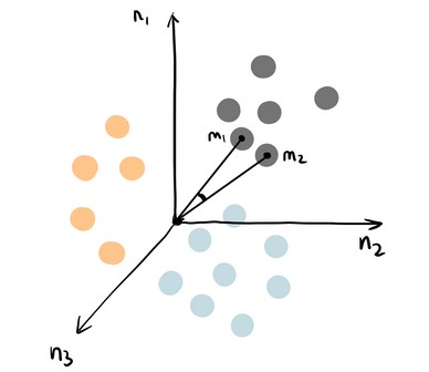
▲knn (image by author)
You can think of k nearest neighbour algorithm as representing each data point in a n dimensional space — which is defined by n features. And it calculates the distance between one point to another, then assign the label of unobserved data based on the labels of nearest observed data points. KNN can also be used for building recommendation system, check out my article on “Collaborative Filtering for Movie Recommendation” if you are interested in this topic.
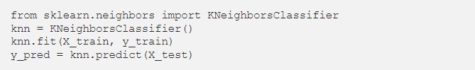
KNN common hyperparameters: n_neighbors, weights, leaf_size, p
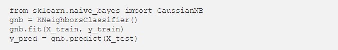
6. Naive Bayes
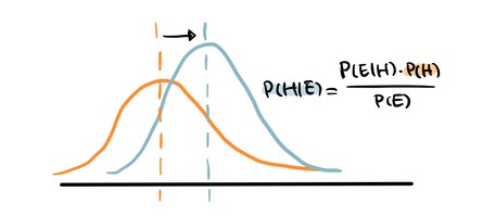
▲naive bayes (image by author)
Naive Bayes is based on Bayes’ Theorem — an approach to calculate conditional probability based on prior knowledge, and the naive assumption that each feature is independent to each other. The biggest advantage of Naive Bayes is that, while most machine learning algorithms rely on large amount of training data, it performs relatively well even when the training data size is small. Gaussian Naive Bayes is a type of Naive Bayes classifier that follows the normal distribution.
gaussian naive bayes common hyperparameters: priors, var_smoothing
Build a Classification Model Pipeline
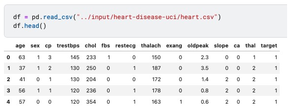
1. Loading Dataset and Data Overview
I chose the popular dataset Heart Disease UCI on Kaggle for predicting the presence of heart disease based on several health related factors.
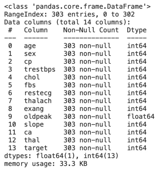
Use df.info()to have a summarized view of dataset, including data type, missing data and number of records.
2. Exploratory Data Analysis (EDA)
Histogram, grouped bar chart and box plot are suitable EDA techniques for classification machine learning algorithms. If you’d like a more comprehensive guide to EDA, please see my post “Semi-Automated Exploratory Data Analysis Process in Python”
Univariate Analysis
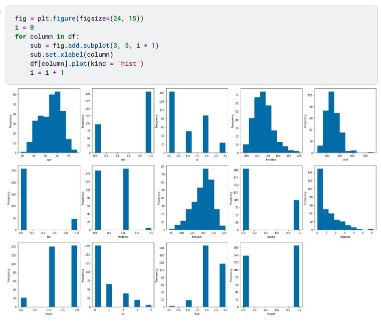
▲univariate analysis (image by author)
Histogram is used for all features, because all features have been encoded into numeric values in the dataset. This saves us the time for categorical encoding that usually happens during the feature engineering stage.
Categorical Features vs. Target — Grouped Bar Chart
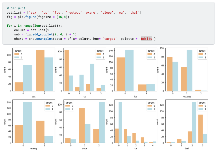
▲grouped bar chart (image by author)
To show how categorical value weigh in determining the target value, grouped bar chart is a straightforward representation. For example, sex = 1 and sex = 0 have distinctly distribution of target value, which indicates it is likely to contribute more to the prediction of target. Contrarily, if the target distribution is the same regardless of the categorical features, then very likely they are not correlated.
Numerical Features vs. Target — Box Plot
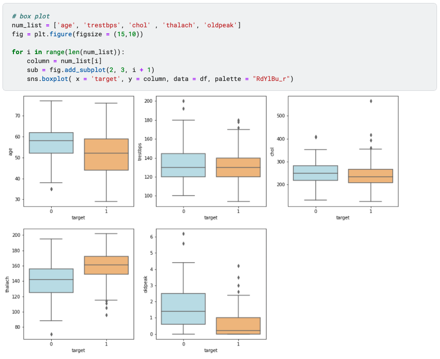
▲box plot (image by author)
Box plot shows how the values of numerical features varies across target groups. For example, we can tell that “oldpeak” have distinct difference when target is 0 vs. target is 1, suggesting that it is an important predictor. However, ‘trestbps’ and ‘chol’ appear to be less outstanding, as the box plot distribution is similar between target groups.
3. Split Dataset into Training and Testing Set
Classification algorithm falls under the category of supervised learning, so dataset needs to be split into a subset for training and a subset for testing (sometime also a validation set). The model is trained on the training set and then examined using the testing set.
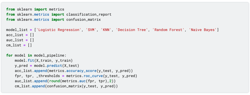
4. Machine Learning Model Pipeline
In order to create a pipeline, I append the default state of all classification algorithms mentioned above into the model list and then iterate through them to train, test, predict and evaluate.
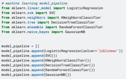
▲model pipeline (image by author)
5. Model Evaluation
▲model evaluation (image by author)
Below is an abstraction explanation of commonly used evaluation methods for classification models — accuracy, ROC & AUC and confusion matrix. Each of the following metrics is worth diving deeper, feel free to visit my article on logistic regression for a more detailed illustration.
1. Accuracy
Accuracy is the most straightforward indicator of the model performance. It measure the percentage of accurate predictions: accuracy = (true positive + true negative) / (true positive + false positive + false negative + false positive)
2. ROC & AUC
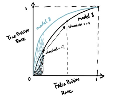
▲ROC & AUC (image by author)
ROC is the plot of true positive rate against false positive rate at various classification threshold. AUC is the area under the ROC curve, and higher AUC indicates better model performance.
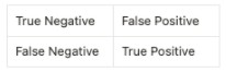
3. Confusion matrix
Confusion matrix indicates the actual values vs. predicted values and summarize the true negative, false positive, false negative and true positive values in a matrix format.
Then we can use seaborn to visualize the confusion matrix in a heatmap.
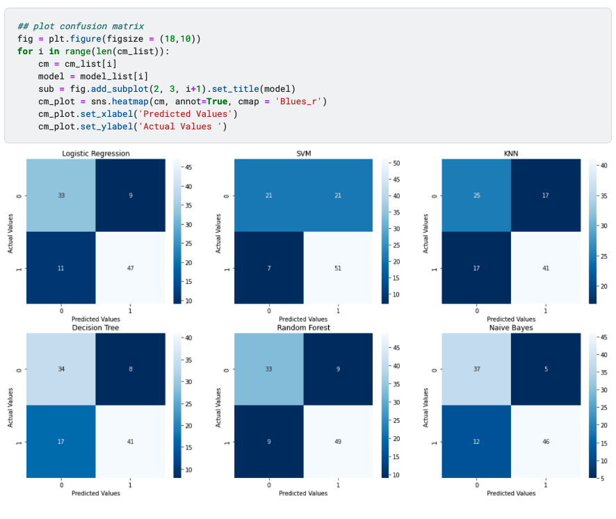
▲confusion matrix plot (image by author)
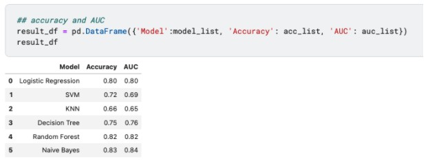
▲accuracy and AUC result (image by author)
Based on three evaluations methods above, random forests and naive bayes have the best performance, whereas KNN is not doing well. However, this doesn’t mean that random forests and naive bayes are superior algorithms. We can only say that they are more suitable for this dataset where the size is relatively smaller and data is not at the same scale.
Each algorithm has its own preference and require different data processing and feature engineering techniques, for example KNN is sensitive to features at difference scale and multicollinearity affects the result of logistic regression. Understanding the characteristics of each allows us to balance the trade-off and select the appropriate model according to the dataset.
轉貼自Source: towardsdatascience.com
若喜歡本文,請關注我們的臉書 Please Like our Facebook Page: Big Data In Finance

留下你的回應
以訪客張貼回應